Two-Dimensional Periodic Hartmann Flow with Electrically Insulating Walls
1. Problem description
This case models incompressible, electrically conducting flow in a two-dimensional channel. The streamwise boundaries are periodic, the top and bottom boundaries are stationary no-slip walls, and those walls are electrically insulating. A uniform transverse magnetic field couples the flow to an inductionless magnetohydrodynamic (MHD) electric-potential equation. A constant streamwise volumetric momentum source drives the flow. Table 1 summarizes the active model choices; every value in the table is taken from the supplied XML input.
Table 1. Active physical and discretization models.
Setting |
Configured value |
|---|---|
Element block |
|
Physics block |
|
Equation-set type |
|
Inductionless MHD equation |
Enabled |
Constant momentum source |
Enabled |
Temperature equation |
Not enabled |
Basis order |
\(1\) |
Integration order |
\(2\) |
The XML hierarchy that activates the models in Table 1 is:
  <ParameterList name="Block ID to Physics ID Mapping">
    <Parameter name="eblock-0_0" type="string" value="FluidPhysicsBlock"/>
  </ParameterList> <!-- Block ID to Physics ID Mapping -->

  <ParameterList name="Physics Blocks">
    <ParameterList name="FluidPhysicsBlock">
      <ParameterList>
        <Parameter name="Type" type="string" value="IncompressibleNavierStokes"/>
        <Parameter name="Basis Order" type="int" value="1"/>
        <Parameter name="Integration Order" type="int" value="2"/>
        <Parameter name="Model ID" type="string" value="fluids"/>
        <Parameter name="Build Constant Source" type="bool" value="true"/>
        <Parameter name="Build Inductionless MHD Equation" type="bool" value="true"/>
      </ParameterList> <!-- -->
    </ParameterList> <!-- FluidPhysicsBlock -->
  </ParameterList> <!-- Physics Blocks -->
Table 2 lists the active physical parameters. Density is not specified in the XML, so the prescribed fallback \(\rho=1.0\ \mathrm{kg\,m^{-3}}\) is assumed and clearly distinguished from extracted input values. The constant source is written as a volumetric momentum source because it enters the conservative momentum residual; its SI unit is therefore \(\mathrm{N\,m^{-3}}\). The inactive constant-flow-rate control and its ancillary target/area entries are retained in the XML excerpt for completeness, but their units are not stated in the source and they are not used because the control is disabled.
Table 2. Physical parameters used by the case.
Quantity |
Symbol |
Value |
|---|---|---|
Kinematic viscosity |
\(\nu\) |
\(0.01\ \mathrm{m^2\,s^{-1}}\) |
Fluid density (assumed fallback) |
\(\rho\) |
\(1.0\ \mathrm{kg\,m^{-3}}\) |
Artificial-compressibility coefficient |
\(\beta\) |
\(100.0\ \mathrm{m^2\,s^{-2}}\) |
Electrical conductivity |
\(\sigma\) |
\(1.0\ \mathrm{S\,m^{-1}}\) |
External magnetic field |
\(\mathbf{B}^{0}\) |
\((0.0,1.0,0.0)\ \mathrm{T}\) |
Volumetric momentum source |
\(\mathbf{s}_{m}\) |
\((4.194528049,0.0)\ \mathrm{N\,m^{-3}}\) |
The exact XML settings represented in Table 2 are:
The density row in Table 2 has no corresponding XML entry because it is the prescribed fallback used only when density is absent; the remaining rows are supported by the following exact settings.
  <ParameterList name="User Data">
    <Parameter name="Output Graph" type="bool" value="false"/>
    <Parameter name="Workset Size" type="int" value="256"/>
    <Parameter name="CFL" type="double" value="100.0"/>
    <Parameter name="CFL_init" type="double" value="1.0"/>
    <Parameter name="CFL_transition" type="double" value="20"/>
    <ParameterList name="External Magnetic Field Parameters">
      <Parameter name="External Magnetic Field Value" type="Array(double)" value="{0.0, 1.0, 0.0}"/>
    </ParameterList> <!-- External Magnetic Field Parameters -->
  </ParameterList> <!-- User Data -->
  <ParameterList name="Closure Models">
    <ParameterList name="fluids">
      <ParameterList name="Fluid Properties">
        <Parameter name="Kinematic viscosity" type="double" value="0.01"/>
        <Parameter name="Artificial compressibility" type="double" value="100.0"/>
        <Parameter name="Electrical conductivity" type="double" value="1.0"/>
        <Parameter name="Build Inductionless MHD Equation" type="bool" value="true"/>
      </ParameterList> <!-- Fluid Properties -->
      <ParameterList name="CONSTANT_SOURCE">
        <Parameter name="Type" type="string" value="IncompressibleConstantSource"/>
        <Parameter name="Momentum Source" type="Array(double)" value="{4.194528049, 0.0}"/>
        <Parameter name="Constant Volumetric Flow Rate" type="bool" value="false"/>
        <Parameter name="Target Volumetric Flow Rate" type="double" value="0.4768116868191465"/>
        <Parameter name="Bottom Wall Surface Area" type="double" value="5.0"/>
        <Parameter name="Inlet Wall Surface Area" type="double" value="2.0"/>
      </ParameterList> <!-- CONSTANT_SOURCE -->
    </ParameterList> <!-- fluids -->
  </ParameterList> <!-- Closure Models -->
Nondimensional project conditions
The project uses the channel half-height \(a=1.0\ \mathrm{m}\) as its single characteristic length. With the uniform initial streamwise speed \(U_c=1.0\ \mathrm{m\,s^{-1}}\), the configured \(\nu=0.01\ \mathrm{m^2\,s^{-1}}\), \(B_0=1.0\ \mathrm{T}\), and \(\sigma=1.0\ \mathrm{S\,m^{-1}}\), together with the prescribed fallback \(\rho=1.0\ \mathrm{kg\,m^{-3}}\), the flow conditions are \(\mathrm{Re}_a=100\) and \(\mathrm{Ha}_a=10\). Equations (6) and (7) give the single definitions and numerical substitutions. A Prandtl number is not applicable because the temperature equation is disabled, as shown in Table 1.
2. Governing equations
The IncompressibleTimeDerivative closure and the configured artificial-compressibility coefficient specify the complete artificial-compressibility (AC) continuity equation. Equation (1) is the AC form used for this case; no EDAC pressure-diffusion closure is selected in the XML.
For the constant-density model, Equation (1) may equivalently be divided by \(\rho\) to give \((\rho\beta)^{-1}\partial p/\partial t+\nabla\cdot\mathbf{u}=0\).
The incompressible momentum balance is given by Equation (2). It contains the constant volumetric source and the Lorentz force, but no buoyancy or other body-force model is enabled.
The inductionless MHD closure uses Ohm’s law, written as Equation (3), to obtain the electric-current density from the electric potential, fluid velocity, and imposed field.
Charge conservation, \(\nabla\cdot\mathbf{J}=0\), converts Equation (3) into the electric-potential equation shown as Equation (4).
The coupling back to Equation (2) is the Lorentz-force density in Equation (5).
Flow conditions
For this plane channel, the characteristic speed is the uniform initial streamwise speed, \(U_c=1.0\ \mathrm{m\,s^{-1}}\), and the sole characteristic length is the channel half-height, \(a=1.0\ \mathrm{m}\). Equation (6) gives the Reynolds number \(\mathrm{Re}_a=100\).
Equation (7) defines the Hartmann number using the same half-height \(a\). With the configured magnetic-field magnitude \(B_0=\lVert\mathbf{B}^{0}\rVert=1.0\ \mathrm{T}\), conductivity \(\sigma=1.0\ \mathrm{S\,m^{-1}}\), viscosity \(\nu=0.01\ \mathrm{m^2\,s^{-1}}\), and prescribed fallback density \(\rho=1.0\ \mathrm{kg\,m^{-3}}\), the Hartmann number is \(\mathrm{Ha}_a=10\).
Table 3 defines every symbol appearing in Equations (1)–(7), including the differential operators. The value of \(\rho\) is the documented fallback assumption because the XML does not specify density.
Table 3. Symbols used in Equations (1)–(7).
Symbol |
Definition |
SI unit |
|---|---|---|
\(t\) |
Time |
\(\mathrm{s}\) |
\(p\) |
Lagrange-pressure field |
\(\mathrm{Pa}\) |
\(\beta\) |
Artificial-compressibility coefficient |
\(\mathrm{m^2\,s^{-2}}\) |
\(\mathbf{u}\) |
Velocity vector |
\(\mathrm{m\,s^{-1}}\) |
\(\rho\) |
Fluid density; assumed as \(1.0\ \mathrm{kg\,m^{-3}}\) because no input value is supplied |
\(\mathrm{kg\,m^{-3}}\) |
\(\nu\) |
Kinematic viscosity |
\(\mathrm{m^2\,s^{-1}}\) |
\(\mathbf{s}_{m}\) |
Constant volumetric momentum source |
\(\mathrm{N\,m^{-3}}\) |
\(\mathbf{J}\) |
Electric-current density |
\(\mathrm{A\,m^{-2}}\) |
\(\mathbf{B}^{0}\) |
Imposed external magnetic field |
\(\mathrm{T}\) |
\(\sigma\) |
Electrical conductivity |
\(\mathrm{S\,m^{-1}}\) |
\(\varphi\) |
Electric potential |
\(\mathrm{V}\) |
\(\mathbf{f}_{L}\) |
Lorentz-force density |
\(\mathrm{N\,m^{-3}}\) |
\(U_c\) |
Characteristic speed, taken as the initial streamwise speed |
\(\mathrm{m\,s^{-1}}\) |
\(a\) |
Channel half-height |
\(\mathrm{m}\) |
\(B_0\) |
Magnitude of the imposed magnetic field, \(\lVert\mathbf{B}^{0}\rVert\) |
\(\mathrm{T}\) |
\(\mathrm{Re}_a\) |
Reynolds number based on \(a\) |
Dimensionless |
\(\mathrm{Ha}_a\) |
Hartmann number based on \(a\) |
Dimensionless |
The exact closure-model selection supporting Equations (1)–(5) is:
  <ParameterList name="Closure Models">
    <ParameterList name="fluids">
      <ParameterList name="DQDT">
        <Parameter name="Type" type="string" value="IncompressibleTimeDerivative"/>
      </ParameterList> <!-- DQDT -->
      <ParameterList name="CONVECTIVE_FLUX">
        <Parameter name="Type" type="string" value="IncompressibleConvectiveFlux"/>
      </ParameterList> <!-- CONVECTIVE_FLUX -->
      <ParameterList name="VISCOUS_FLUX">
        <Parameter name="Type" type="string" value="IncompressibleViscousFlux"/>
      </ParameterList> <!-- VISCOUS_FLUX -->
      <ParameterList name="EP_DIFFUSION">
        <Parameter name="Type" type="string" value="ElectricPotentialDiffusionFlux"/>
      </ParameterList> <!-- EP_DIFFUSION -->
      <ParameterList name="EP_CROSS_PRODUCT">
        <Parameter name="Type" type="string" value="ElectricPotentialCrossProductFlux"/>
      </ParameterList> <!-- EP_CROSS_PRODUCT -->
      <ParameterList name="ext_magn_field">
        <Parameter name="Type" type="string" value="ExternalMagneticField"/>
      </ParameterList> <!-- ext_magn_field -->
      <ParameterList name="elec_current_density">
        <Parameter name="Type" type="string" value="ElectricCurrentDensity"/>
      </ParameterList> <!-- elec_current_density -->
      <ParameterList name="lorentz_force">
        <Parameter name="Type" type="string" value="LorentzForce"/>
      </ParameterList> <!-- lorentz_force -->
    </ParameterList> <!-- fluids -->
  </ParameterList> <!-- Closure Models -->
3. Geometry and mesh description
The XML defines an inline rectangular domain \(0.0\ \mathrm{m}\leq x\leq5.0\ \mathrm{m}\) and \(-1.0\ \mathrm{m}\leq y\leq1.0\ \mathrm{m}\). It is divided into one block containing \(8\times32=256\) four-node quadrilateral (Quad4) elements. Thus the uniform element dimensions are \(\Delta x=0.625\ \mathrm{m}\) and \(\Delta y=0.0625\ \mathrm{m}\). Table 4 records the mesh values, and Figure 1 visualizes the resulting structured mesh and boundary types.
Table 4. Inline geometry and mesh.
Quantity |
Value |
|---|---|
Streamwise interval |
\(x\in[0.0,5.0]\ \mathrm{m}\) |
Wall-normal interval |
\(y\in[-1.0,1.0]\ \mathrm{m}\) |
Domain length |
\(5.0\ \mathrm{m}\) |
Domain height |
\(2.0\ \mathrm{m}\) |
Element type |
|
Number of elements in \(x\) |
\(8\) |
Number of elements in \(y\) |
\(32\) |
Total number of elements |
\(256\) |
Number of mesh blocks in each direction |
\(1\times1\) |
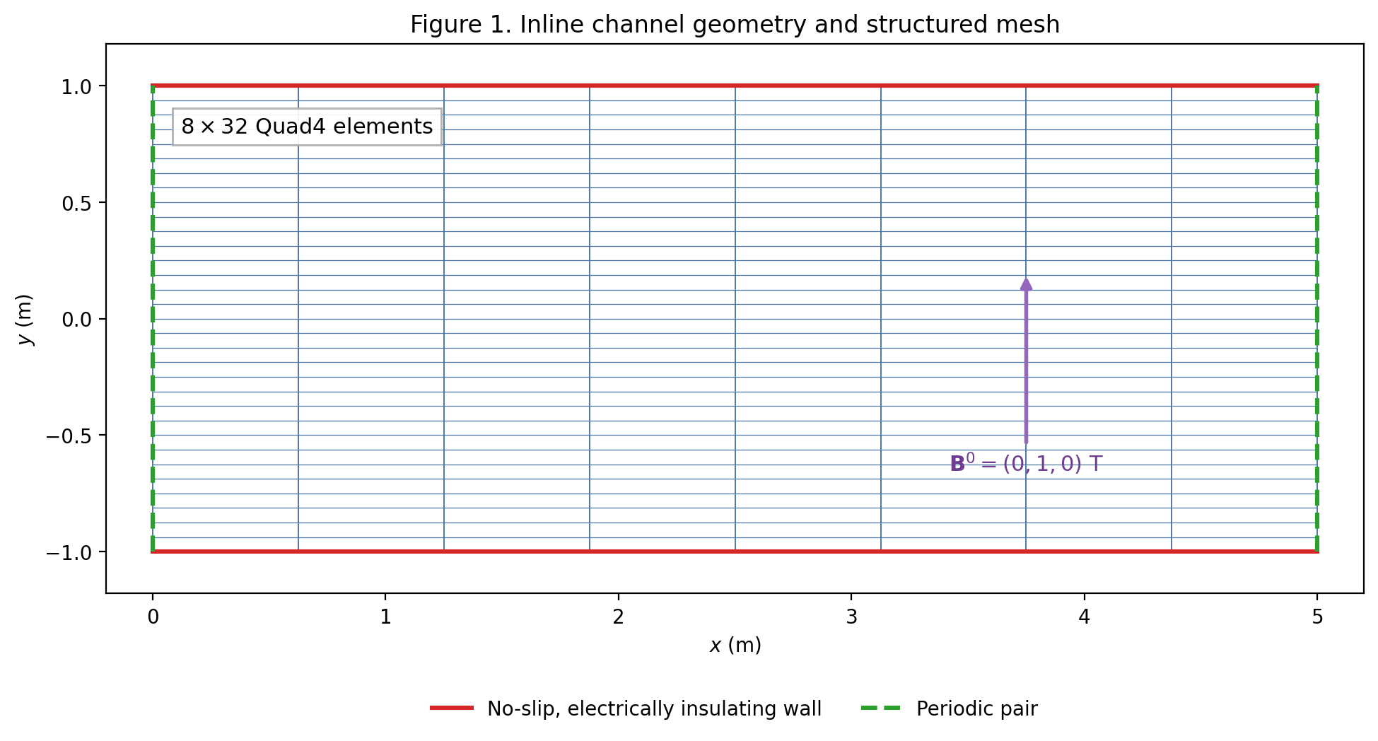
Figure 1 is generated from the inline mesh definition below. The left and right sides are paired with the y-all periodic condition using a geometric matching tolerance of \(10^{-8}\ \mathrm{m}\). No Exodus mesh file was supplied, so Exodus-specific node numbering, side-set IDs, and connectivity beyond the inline structured definition cannot be independently checked.
  <ParameterList name="Mesh">
    <Parameter name="Mesh Input Type" type="string" value="Inline"/>
    <ParameterList name="Inline">
      <Parameter name="Element Type" type="string" value="Quad4"/>
      <ParameterList name="Mesh">
        <Parameter name="X Blocks" type="int" value="1"/>
        <Parameter name="Y Blocks" type="int" value="1"/>
        <Parameter name="X Elements" type="int" value="8"/>
        <Parameter name="Y Elements" type="int" value="32"/>
        <Parameter name="X0" type="double" value="0.0"/>
        <Parameter name="Y0" type="double" value="-1.0"/>
        <Parameter name="Xf" type="double" value="5.0"/>
        <Parameter name="Yf" type="double" value="1.0"/>
        <ParameterList name="Periodic BCs">
          <Parameter name="Count" type="int" value="1"/>
          <Parameter name="Periodic Condition 1" type="string" value="y-all 1e-8: left;right"/>
        </ParameterList> <!-- Periodic BCs -->
      </ParameterList> <!-- Mesh -->
    </ParameterList> <!-- Inline -->
  </ParameterList> <!-- Mesh -->
4. Initial and boundary conditions
The fields are initialized uniformly over eblock-0_0. Table 5 shows the initial values: zero Lagrange pressure, unit streamwise velocity, zero wall-normal velocity, and a constant electric potential.
Table 5. Uniform initial conditions.
Field |
Initial value |
|---|---|
Lagrange pressure, \(p(\mathbf{x},0)\) |
\(0.0\ \mathrm{Pa}\) |
Streamwise velocity, \(u_x(\mathbf{x},0)\) |
\(1.0\ \mathrm{m\,s^{-1}}\) |
Wall-normal velocity, \(u_y(\mathbf{x},0)\) |
\(0.0\ \mathrm{m\,s^{-1}}\) |
Electric potential, \(\varphi(\mathbf{x},0)\) |
\(2.0\ \mathrm{V}\) |
In Table 5, \(\mathbf{x}=(x,y)\) is the position vector with SI unit \(\mathrm{m}\). The exact initial-condition syntax is:
  <ParameterList name="Initial Conditions">
    <ParameterList name="eblock-0_0">
      <ParameterList name="Constant Lagrange Pressure">
        <Parameter name="Type" type="string" value="Constant"/>
        <Parameter name="Equation Set Name" type="string" value="lagrange_pressure"/>
        <Parameter name="Value" type="double" value="0.0"/>
      </ParameterList> <!-- Constant Lagrange Pressure -->
      <ParameterList name="Constant Velocity 0">
        <Parameter name="Type" type="string" value="Constant"/>
        <Parameter name="Equation Set Name" type="string" value="velocity_0"/>
        <Parameter name="Value" type="double" value="1.0"/>
      </ParameterList> <!-- Constant Velocity 0 -->
      <ParameterList name="Constant Velocity 1">
        <Parameter name="Type" type="string" value="Constant"/>
        <Parameter name="Equation Set Name" type="string" value="velocity_1"/>
        <Parameter name="Value" type="double" value="0.0"/>
      </ParameterList> <!-- Constant Velocity 1 -->
      <ParameterList name="Constant Electric Potential">
        <Parameter name="Type" type="string" value="Constant"/>
        <Parameter name="Equation Set Name" type="string" value="electric_potential"/>
        <Parameter name="Value" type="double" value="2.0"/>
      </ParameterList> <!-- Constant Electric Potential -->
    </ParameterList> <!-- eblock-0_0 -->
  </ParameterList> <!-- Initial Conditions -->
At \(y=1.0\ \mathrm{m}\) (top) and \(y=-1.0\ \mathrm{m}\) (bottom), the No-Slip condition sets the stationary-wall velocity to \(\mathbf{u}=\mathbf{0}\ \mathrm{m\,s^{-1}}\). ElectricCurrentDensityInsulating imposes zero normal current, summarized by Equation (8), where \(\mathbf{n}\) is the outward unit normal and is dimensionless.
The left and right sides are periodic, as specified in the mesh excerpt in Section 3. The exact wall-condition syntax supporting Equation (8) is:
  <ParameterList name="Boundary Conditions">
    <ParameterList>
      <Parameter name="Sideset ID" type="string" value="top, bottom"/>
      <Parameter name="Element Block ID" type="string" value="eblock-0_0"/>
      <Parameter name="Strategy" type="string" value="IncompressibleBoundaryFlux"/>
      <ParameterList name="Data">
        <ParameterList name="Navier-Stokes">
          <Parameter name="Type" type="string" value="No-Slip"/>
        </ParameterList> <!-- Navier-Stokes -->
        <ParameterList name="Electric Potential">
          <Parameter name="Type" type="string" value="ElectricCurrentDensityInsulating"/>
        </ParameterList> <!-- Electric Potential -->
      </ParameterList> <!-- Data -->
    </ParameterList> <!-- -->
  </ParameterList> <!-- Boundary Conditions -->
5. Solver configuration and convergence criteria
The spatial discretization uses first-order basis functions with second-order integration, as shown in the physics-block excerpt in Section 1. Time integration uses Backward Euler and a constant step-control mode. The configured interval is \(0.0\ \mathrm{s}\) to \(10000.0\ \mathrm{s}\) with a maximum of \(100\) time indices. The initial and minimum time steps are both \(0.0001\ \mathrm{s}\), while the maximum is \(100.0\ \mathrm{s}\). Table 6 consolidates the nonlinear and linear solver choices and convergence limits.
Table 6. Time-integration and solver configuration.
Category |
Setting |
Value |
|---|---|---|
Time integration |
Stepper |
Backward Euler |
Time integration |
Initial/final time |
\(0.0/10000.0\ \mathrm{s}\) |
Time integration |
Final time index |
\(100\) |
Time integration |
Minimum/initial/maximum step |
\(0.0001/0.0001/100.0\ \mathrm{s}\) |
Time integration |
Step-control mode |
Constant |
Time integration |
Maximum absolute/relative error |
\(10^{-8}/10^{-8}\) |
Nonlinear solver |
Method |
Newton, line-search based, full step |
Nonlinear solver |
Residual test |
\(\lVert\mathbf{F}\rVert_2\leq10^{-11}\) |
Nonlinear solver |
Maximum Newton iterations |
\(10\) |
Nonlinear solver |
Test combination |
OR |
Linear solver |
Solver |
Belos |
Linear solver |
Preconditioner |
Ifpack2 Schwarz, overlap level \(1\) |
Subdomain solve |
Solver |
Amesos2 Tacho LU |
Execution |
Workset size |
\(256\) |
Pseudo-time control |
Initial/target CFL number |
\(1.0/100.0\) |
Pseudo-time control |
CFL transition |
\(20\) |
Here \(\mathbf{F}\) is the assembled nonlinear residual vector; the XML does not define a physical SI unit for its combined norm, so the configured norm threshold in Table 6 is reported as a solver scalar. The absolute and relative error thresholds are likewise reported exactly as configured rather than assigned invented physical units. The CFL numbers, polynomial orders, iteration counts, overlap level, workset size, and time index are dimensionless.
The linear-solver and preconditioner settings in Table 6 come from:
  <ParameterList name="Linear Solver">
    <Parameter name="Linear Solver Type" type="string" value="Belos"/>
    <Parameter name="Preconditioner Type" type="string" value="Ifpack2"/>
    <ParameterList name="Linear Solver Types">
      <ParameterList name="Belos">
        <ParameterList name="VerboseObject">
          <Parameter name="Verbosity Level" type="string" value="none"/>
        </ParameterList> <!-- VerboseObject -->
      </ParameterList> <!-- Belos -->
    </ParameterList> <!-- Linear Solver Types -->
    <ParameterList name="Preconditioner Types">
      <ParameterList name="Ifpack2">
        <Parameter name="Prec Type" type="string" value="SCHWARZ"/>
        <ParameterList name="Ifpack2 Settings">
          <Parameter name="schwarz: overlap level" type="int" value="1"/>
          <Parameter name="subdomain solver name" type="string" value="Amesos2"/>
          <ParameterList name="subdomain solver parameters">
            <Parameter name="Amesos2 solver name" type="string" value="tacho"/>
            <ParameterList name="Amesos2">
              <ParameterList name="Tacho">
                <Parameter name="method" type="string" value="lu"/>
              </ParameterList> <!-- Tacho -->
            </ParameterList> <!-- Amesos2 -->
          </ParameterList> <!-- subdomain solver parameters -->
        </ParameterList> <!-- Ifpack2 Settings -->
      </ParameterList> <!-- Ifpack2 -->
    </ParameterList> <!-- Preconditioner Types -->
  </ParameterList> <!-- Linear Solver -->
The time-control settings in Table 6 are:
  <ParameterList name="Tempus">
    <Parameter name="Integrator Name" type="string" value="Default Integrator"/>
    <ParameterList name="Default Integrator">
      <Parameter name="Integrator Type" type="string" value="Integrator Basic"/>
      <Parameter name="Stepper Name" type="string" value="Default Stepper"/>
      <ParameterList name="Solution History">
        <Parameter name="Storage Type" type="string" value="Undo"/>
        <Parameter name="Storage Limit" type="int" value="2"/>
      </ParameterList> <!-- Solution History -->
      <ParameterList name="Time Step Control">
        <Parameter name="Initial Time" type="double" value="0.0"/>
        <Parameter name="Final Time" type="double" value="10000.0"/>
        <Parameter name="Final Time Index" type="int" value="100"/>
        <Parameter name="Minimum Time Step" type="double" value="0.0001"/>
        <Parameter name="Initial Time Step" type="double" value="0.0001"/>
        <Parameter name="Maximum Time Step" type="double" value="100.0"/>
        <Parameter name="Minimum Order" type="int" value="1"/>
        <Parameter name="Initial Order" type="int" value="1"/>
        <Parameter name="Maximum Order" type="int" value="2"/>
        <Parameter name="Maximum Absolute Error" type="double" value="1.0e-8"/>
        <Parameter name="Maximum Relative Error" type="double" value="1.0e-8"/>
        <Parameter name="Integrator Step Type" type="string" value="Constant"/>
        <Parameter name="Maximum Number of Stepper Failures" type="int" value="10"/>
        <Parameter name="Maximum Number of Consecutive Stepper Failures" type="int" value="5"/>
      </ParameterList> <!-- Time Step Control -->
    </ParameterList> <!-- Default Integrator -->
    <ParameterList name="Default Stepper">
      <Parameter name="Stepper Type" type="string" value="Backward Euler"/>
      <Parameter name="Solver Name" type="string" value="Default Solver"/>
      <Parameter name="Zero Initial Guess" type="bool" value="false"/>
The Newton convergence criteria completing that hierarchy are:
      <ParameterList name="Default Solver">
        <ParameterList name="NOX">
          <ParameterList name="Direction">
            <Parameter name="Method" type="string" value="Newton"/>
            <ParameterList name="Newton">
              <Parameter name="Forcing Term Method" type="string" value="Constant"/>
              <Parameter name="Rescue Bad Newton Solve" type="bool" value="1"/>
              <ParameterList name="Stratimikos Linear Solver">
                <ParameterList name="NOX Stratimikos Options">
                </ParameterList>
              </ParameterList> <!-- Stratimikos Linear Solver -->
            </ParameterList> <!-- Newton -->
          </ParameterList> <!-- Direction -->
          <ParameterList name="Line Search">
            <Parameter name="Method" type="string" value="Full Step"/>
            <ParameterList name="Full Step">
              <Parameter name="Full Step" type="double" value="1"/>
            </ParameterList> <!-- Full Step -->
          </ParameterList> <!-- Line Search -->
          <Parameter name="Nonlinear Solver" type="string" value="Line Search Based"/>
          <ParameterList name="Solver Options">
            <Parameter name="Status Test Check Type" type="string" value="Minimal"/>
          </ParameterList> <!-- Solver Options -->
          <ParameterList name="Status Tests">
            <Parameter name="Test Type" type="string" value="Combo"/>
            <Parameter name="Combo Type" type="string" value="OR"/>
            <Parameter name="Number of Tests" type="int" value="2"/>
            <ParameterList name="Test 0">
              <Parameter name="Test Type" type="string" value="NormF"/>
              <Parameter name="Tolerance" type="double" value="1.0e-11"/>
            </ParameterList> <!-- Test 0 -->
            <ParameterList name="Test 1">
              <Parameter name="Test Type" type="string" value="MaxIters"/>
              <Parameter name="Maximum Iterations" type="int" value="10"/>
            </ParameterList> <!-- Test 1 -->
          </ParameterList> <!-- Status Tests -->
        </ParameterList> <!-- NOX -->
      </ParameterList> <!-- Default Solver -->
    </ParameterList> <!-- Default Stepper -->
  </ParameterList> <!-- Tempus -->
The local-step and CFL-related controls referred to in Table 6 are selected by:
  <ParameterList name="User Data">
    <Parameter name="Workset Size" type="int" value="256"/>
    <Parameter name="CFL" type="double" value="100.0"/>
    <Parameter name="CFL_init" type="double" value="1.0"/>
    <Parameter name="CFL_transition" type="double" value="20"/>
  </ParameterList> <!-- User Data -->
  <ParameterList name="Closure Models">
    <ParameterList name="fluids">
      <ParameterList name="element_length">
        <Parameter name="Type" type="string" value="ElementLength"/>
      </ParameterList> <!-- element_length -->
      <ParameterList name="local_time_step_size">
        <Parameter name="Type" type="string" value="IncompressibleLocalTimeStepSize"/>
      </ParameterList> <!-- local_time_step_size -->
    </ParameterList> <!-- fluids -->
  </ParameterList> <!-- Closure Models -->
6. Numerical results
Numerical results of the Hartmann problem obtained using Vertex-CFD are presented in Figures 2 and 3. The computed velocity profile is nearly uniform in the central region of the domain, while sharp velocity gradients develop near the walls, commonly referred to as Hartmann walls. As the Hartmann number, \(Ha\), increases, the core flow becomes progressively flatter and the near-wall boundary layers become thinner. In particular, the characteristic boundary-layer thickness, \(\delta\), is inversely proportional to the Hartmann number, such that \(\delta \propto Ha^{-1}\).
The Hartmann problem admits an analytical solution that can be derived from the momentum equation under the assumption of a steady, fully developed flow. This solution provides a suitable benchmark for assessing the accuracy of the numerical method. Accordingly, error norms are computed by comparing the numerical and analytical velocity profiles at different mesh resolutions. The corresponding convergence orders are also reported to evaluate the rate at which the numerical solution approaches the analytical solution under mesh refinement.
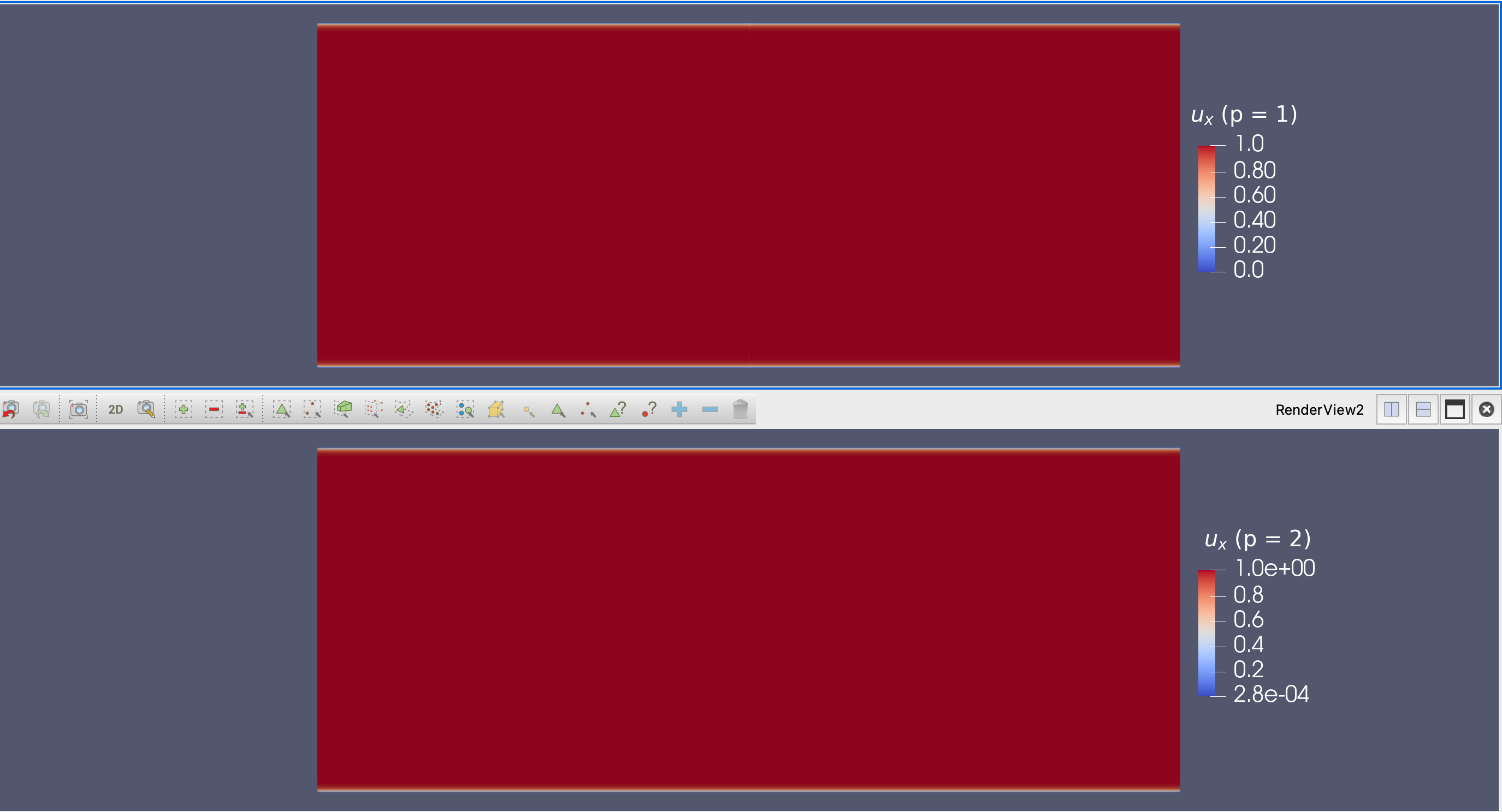
Figure 2. Velocity surface plots for \(Re = 100\) and \(H_a = 100\) with linear and quadratic basis functions.
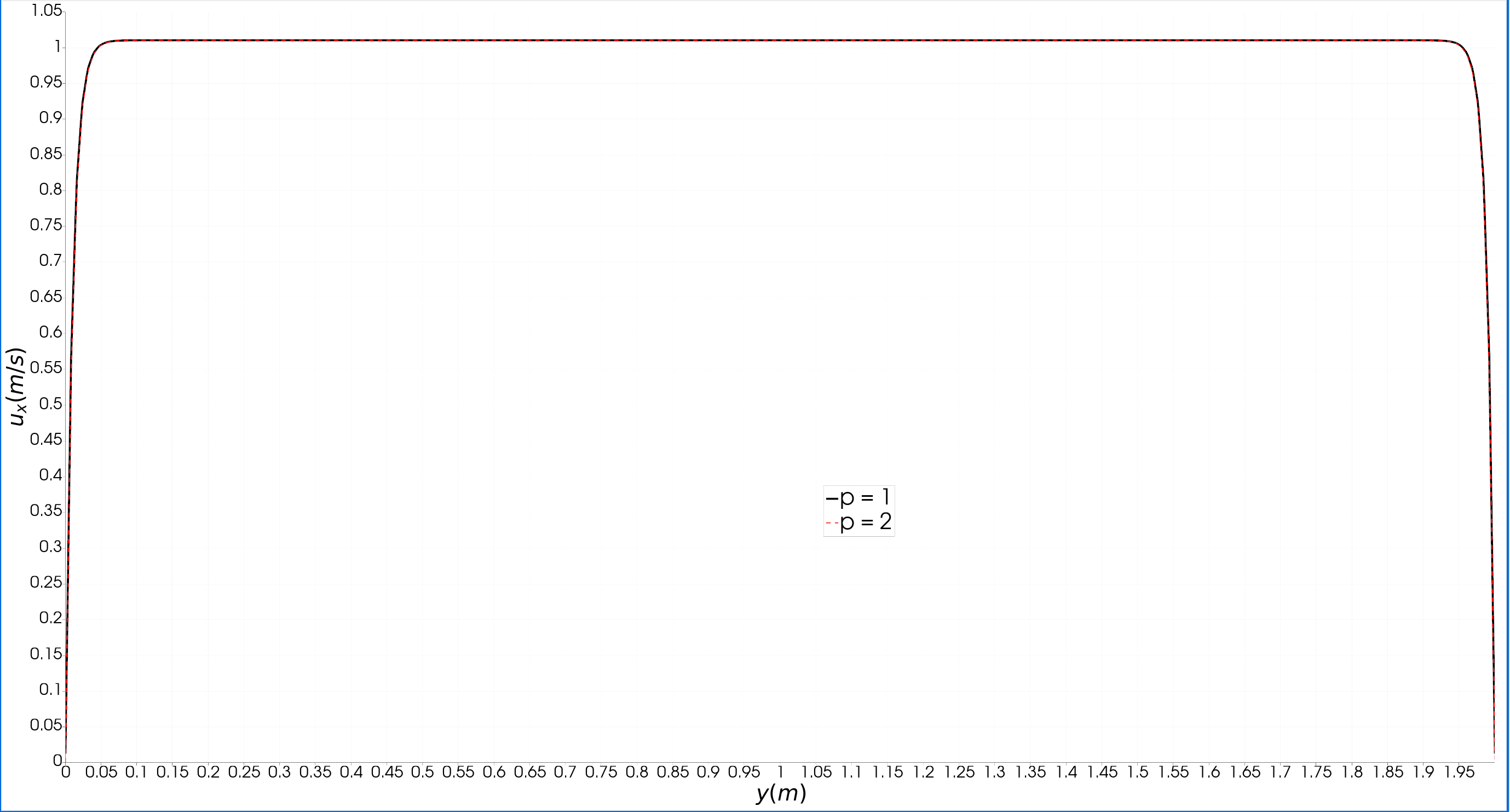
Figure 3. Velocity line plots for \(Re = 100\) and \(H_a = 100\) with linear and quadratic basis functions.
The analytical solution for the velocity is a function of the Hartmann number \(H_a\):
where
The flow is driven by a pressure drop imposed through a volumetric source term. The linear pressure drop \(\frac{dp}{dx}\) is a function of the Hartmann number \(H_a\), the Reynolds number \(Re\), and the surface-averaged velocity \(U\):
where
For a Reynolds number of \(100\), the linear pressure drop is computed, and the resulting values are shown in Table 1.
Case |
\(Re\) |
\(H_a\) |
\(\dfrac{dp}{dx}\) |
|---|---|---|---|
1 |
100 |
100 |
101.010101 |
An \(h\)-refinement and \(p\)-refinement study was performed for the two cases in Table 1 using a channel uniformly meshed with quadrilateral and triangular elements. The \(L_1\) error norm between the numerical surface-averaged velocity and its exact solution, \(U=1.0\ \mathrm{m/s}\), was computed.
The results and corresponding orders of convergence are reported in Table 2, Table 3.Second-order accuracy is achieved when linear basis functions are used. With quadratic basis functions, the observed convergence order exceeds three, indicating superconvergent behavior. Such behavior may occur for problems characterized by strong localized gradients, such as those present within the thin Hartmann boundary layers.
\(N_y\) |
\(L_1\) error norm (quads) |
Order (quads) |
\(L_1\) error norm (tris) |
Order (tris) |
|---|---|---|---|---|
128 |
0.000535586 |
— |
0.000534261 |
— |
256 |
0.000132993 |
2.009767951 |
0.000132622 |
2.010220367 |
512 |
\(3.13744\times10^{-5}\) |
2.083692812 |
\(3.12732\times10^{-5}\) |
2.084323335 |
1024 |
\(7.45231\times10^{-6}\) |
2.073826005 |
\(7.42561\times10^{-6}\) |
2.074346137 |
\(N_y\) |
\(L_1\) error norm (quads) |
Order (quads) |
\(L_1\) error norm (tris) |
Order (tris) |
|---|---|---|---|---|
64 |
0.000226979 |
— |
0.000209159 |
— |
80 |
0.000104845 |
3.461329866 |
\(9.47078\times10^{-5}\) |
3.550615033 |
96 |
\(5.1625\times10^{-5}\) |
3.885878924 |
\(4.54439\times10^{-5}\) |
4.027599172 |
128 |
\(1.39733\times10^{-5}\) |
4.021815589 |
\(1.12814\times10^{-5}\) |
4.843266273 |