3D Incompressible Rayleigh-Benard Convection Tutorial

This tutorial documents the input deck incompressible_3d_rayleigh_benard_convection.xml and the associated Exodus mesh 3d_rayleigh_benard.exo. The case models buoyancy-driven convection of an incompressible fluid confined between a heated bottom wall and a cooled top wall inside a cylindrical enclosure — the classical Rayleigh–Bénard configuration.

---

1. Problem description

The simulation solves for the transient, three-dimensional flow of a single-phase incompressible fluid enclosed in a right circular cylinder. The fluid is at rest initially and is subsequently driven into convective motion by a temperature difference imposed between the bottom (hot) and top (cold) end walls, with gravity \(\mathbf{g}\) acting along the negative \(z\)-direction (axis of the cylinder). The lateral wall of the cylinder is adiabatic and no-slip, so that heat can only enter and leave the domain through the bottom and top disks.

The physics is built from the IncompressibleNavierStokes physics block with the temperature equation and the Boussinesq buoyancy source both enabled (Build Temperature Equation = true, Build Buoyancy Source = true), and the continuity constraint is enforced through an Entropically Damped Artificial Compressibility (EDAC) formulation rather than a classical projection/pressure-Poisson approach. This choice, together with the fluid properties and boundary temperatures, fixes the Prandtl and Rayleigh numbers of the problem, discussed in Section 2.

The XML snippet below shows how the physics is attached to the single element block (block-1) present in the mesh:

<ParameterList name="Block ID to Physics ID Mapping">
  <Parameter name="block-1" type="string" value="FluidPhysicsBlock"/>
</ParameterList>

<ParameterList name="Physics Blocks">
  <ParameterList name="FluidPhysicsBlock">
    <ParameterList>
      <Parameter name="Type" type="string" value="IncompressibleNavierStokes"/>
      <Parameter name="Basis Order" type="int" value="1"/>
      <Parameter name="Integration Order" type="int" value="2"/>
      <Parameter name="Model ID" type="string" value="fluids"/>
      <Parameter name="Build Temperature Equation" type="bool" value="true"/>
      <Parameter name="Build Buoyancy Source" type="bool" value="true"/>
    </ParameterList>
  </ParameterList>
</ParameterList>

---

2. Governing equations

The fluid is modeled as incompressible with constant transport properties under the Boussinesq approximation (density variations are retained only in the buoyancy term). Three fields are solved: velocity \(\mathbf{u}\), a Lagrange/kinematic pressure \(p\), and temperature \(T\).

2.1 Momentum equation

\[ \frac{\partial \mathbf{u}}{\partial t} + (\mathbf{u}\cdot\nabla)\mathbf{u} = -\nabla p + \nu \nabla^{2}\mathbf{u} + \alpha_{th}\,(T - T_{ref})\,\mathbf{g} \]

where \(\nu\) is the kinematic viscosity, \(\alpha_{th}\) is the thermal expansion coefficient, \(T_{ref}\) is the reference temperature about which the Boussinesq buoyancy term is linearized, and \(\mathbf{g}\) is the gravitational acceleration vector. The last term is built by the IncompressibleBuoyancySource closure model.

2.2 Continuity equation (EDAC)

The Continuity Model parameter in the Fluid Properties closure model is set to EDAC, so the divergence-free constraint \(\nabla\cdot\mathbf{u}=0\) is replaced by an evolution equation for the pressure that entropically damps pressure fluctuations while remaining consistent with the incompressible limit as the artificial compressibility coefficient becomes large:

\[ \frac{\partial p}{\partial t} + \mathbf{u}\cdot\nabla p + \beta\,\nabla\cdot\mathbf{u} = \nu\,\nabla^{2} p \]

Here \(\beta\) is the artificial compressibility coefficient (Artificial compressibility in the input file), which plays the role of a pseudo-acoustic wave speed squared, and the right-hand side diffusion term uses the fluid kinematic viscosity \(\nu\) as the entropic damping diffusivity, consistent with the standard EDAC formulation. As \(\beta \to \infty\) this equation degenerates to \(\nabla\cdot\mathbf{u}=0\), recovering the incompressible constraint; for finite \(\beta\) it acts as a stabilized pseudo-time relaxation toward that constraint. Table 1 reports the value of \(\beta\) used in this case.

2.3 Energy equation

\[ \frac{\partial T}{\partial t} + \mathbf{u}\cdot\nabla T = \kappa\,\nabla^{2}T, \qquad \kappa = \frac{k}{\rho\,c_p} \]

where \(k\) is the thermal conductivity, \(\rho\) the density, and \(c_p\) the specific heat capacity, so that \(\kappa\) is the thermal diffusivity.

2.4 Fluid properties and dimensionless groups

Table 1 lists the fluid properties as specified in the Fluid Properties closure model.

Table 1. Fluid properties used in the fluids closure model.

Quantity	Symbol	Value	Units
Kinematic viscosity	\(\nu\)	\(0.1\)	\(\mathrm{m^2/s}\)
Density	\(\rho\)	\(1.0\)	\(\mathrm{kg/m^3}\)
Thermal conductivity	\(k\)	\(1.0\)	\(\mathrm{W/(m \cdot K)}\)
Specific heat capacity	\(c_p\)	\(70.0\)	\(\mathrm{J/(kg \cdot K)}\)
Artificial compressibility coefficient	\(\beta\)	\(1.0\times10^{5}\)	\(\mathrm{m^2/s^2}\)
Thermal expansion coefficient	\(\alpha_{th}\)	\(0.014285715\)	\(\mathrm{K^{-1}}\)
Reference temperature	\(T_{ref}\)	\(200.0\)	\(\mathrm{K}\)
Heat capacity ratio	\(\gamma\)	\(1.0\)	—
Continuity model	—	EDAC	—

From these values, the thermal diffusivity is \(\kappa = k/(\rho c_p) = 1.0/(1.0\times70.0) \approx 0.01429\ \mathrm{m^2/s}\), giving a Prandtl number

\[ Pr = \frac{\nu}{\kappa} = \frac{0.1}{0.01429} \approx 7.0 \]

The Rayleigh number, based on the wall-to-wall temperature difference \(\Delta T = T_{bottom}-T_{top}=50.0\ \mathrm{K}\) (Section 4) and the cylinder height \(H\) (Section 3), is

\[ Ra = \frac{|\mathbf{g}|\,\alpha_{th}\,\Delta T\, H^{3}}{\nu\,\kappa} \approx 5.0\times10^{3}\, H^{3} \]

with \(H\) expressed in meters. The exact value of \(Ra\) therefore depends on the cylinder height read from the mesh coordinate data (Table 2); the formula is reported here so it can be evaluated once \(H\) is confirmed from the Exodus file.

The syntax used to define these properties and the continuity model is:

<ParameterList name="Fluid Properties">
  <Parameter name="Build Temperature Equation" type="bool" value="true"/>
  <Parameter name="Build Buoyancy Source" type="bool" value="true"/>
  <Parameter name="Kinematic viscosity" type="double" value="0.1"/>
  <Parameter name="Density" type="double" value="1.0"/>
  <Parameter name="Thermal conductivity" type="double" value="1.0"/>
  <Parameter name="Specific heat capacity" type="double" value="70.0"/>
  <Parameter name="Artificial compressibility" type="double" value="100000.0"/>
  <Parameter name="Expansion coefficient" type="double" value="0.014285715"/>
  <Parameter name="Reference temperature" type="double" value="200.0"/>
  <Parameter name="Continuity Model" type="string" value="EDAC"/>
  <Parameter name="Heat capacity ratio" type="double" value="1.0"/>
</ParameterList>

The remaining closure models assemble the discrete terms of the equations above from the physics block: DQDT (time derivative), CONVECTIVE_FLUX and VISCOUS_FLUX (momentum flux terms), BUOYANCY_SOURCE (buoyancy term), together with two auxiliary models used for time-step control, element_length and local_time_step_size, and a scalar response model nusselt_number used for output (Section 6):

<ParameterList name="DQDT">
  <Parameter name="Type" type="string" value="IncompressibleTimeDerivative"/>
</ParameterList>
<ParameterList name="CONVECTIVE_FLUX">
  <Parameter name="Type" type="string" value="IncompressibleConvectiveFlux"/>
</ParameterList>
<ParameterList name="VISCOUS_FLUX">
  <Parameter name="Type" type="string" value="IncompressibleViscousFlux"/>
</ParameterList>
<ParameterList name="BUOYANCY_SOURCE">
  <Parameter name="Type" type="string" value="IncompressibleBuoyancySource"/>
</ParameterList>

No electric potential or electromagnetic equation is present in this input file (the physics block is purely hydro-thermal), so no such field appears in Section 6.

---

3. Geometry and mesh description

The computational domain is a right circular cylinder of radius \(R\) and height \(H\), with its axis aligned with the (vertical) \(z\)-direction along which gravity acts. Figure 1 shows a schematic of the domain together with the three named surfaces used to apply boundary conditions: the bottom disk (hot, heated wall), the top disk (cold wall), and the wall (adiabatic lateral surface).

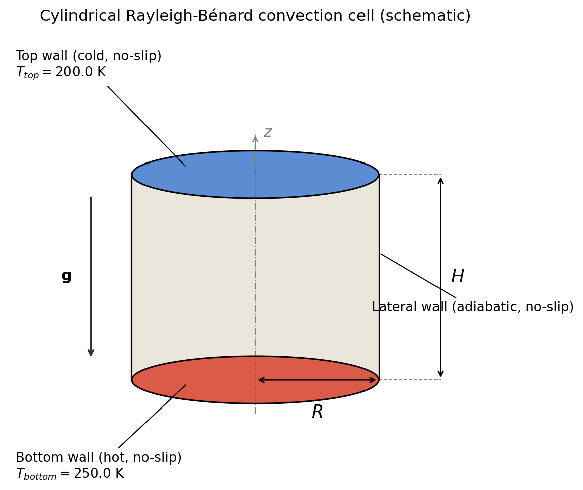
Figure 1. Schematic of the cylindrical convection cell (not to scale). The bottom disk is held at the hot wall temperature, the top disk at the cold wall temperature, and the lateral surface is adiabatic. Gravity \(\mathbf{g}\) points from the cold to the hot wall, i.e. the layer is heated from below.

The mesh is stored in the Exodus file 3d_rayleigh_benard.exo, generated with CUBIT and referenced by the input deck as follows:

<ParameterList name="Mesh">
  <Parameter name="Mesh Input Type" type="string" value="File"/>
  <ParameterList name="File">
    <Parameter name="File Name" type="string" value="3d_rayleigh_benard.exo"/>
    <Parameter name="Decomp Method" type="string" value="GEOM_KWAY"/>
  </ParameterList>
</ParameterList>

Inspection of the Exodus/netCDF4 metadata shows a single all-hexahedral (HEX8, trilinear) element block, block-1, extruded uniformly along \(z\) from a circular footprint, and three side sets that match the three boundary-condition entries of the input file. The resulting mesh statistics are summarized in Table 2, and a schematic of the mesh topology (footprint and extrusion) is shown in Figure 2.

Table 2. Mesh statistics extracted from 3d_rayleigh_benard.exo.

Quantity	Value
Element topology	HEX8 (linear hexahedron)
Spatial dimension	3
Number of element blocks	1 (block-1)
Number of elements	1568
Number of nodes	1944
Number of vertically extruded layers	7
Number of side sets	3 (top, bottom, wall)
Faces on top side set	224
Faces on bottom side set	224
Faces on wall side set	252

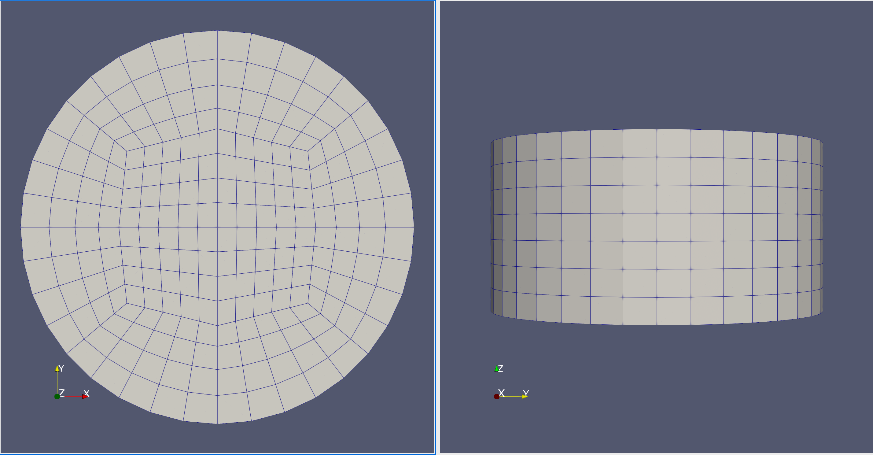
Figure 2. Mesh view extracted from 3d_rayleigh_benard.exo.

---

4. Initial and boundary conditions

4.1 Boundary conditions

Three boundary conditions are applied through the IncompressibleBoundaryFlux strategy, one per side set, as summarized in Table 3.

Table 3. Boundary conditions applied on block-1.

Side set	Velocity condition	Thermal condition
top	No-slip (\(\mathbf{u}=\mathbf{0}\))	Fixed temperature, \(T_{top}=200.0\ \mathrm{K}\)
bottom	No-slip (\(\mathbf{u}=\mathbf{0}\))	Fixed temperature, \(T_{bottom}=250.0\ \mathrm{K}\)
wall	No-slip (\(\mathbf{u}=\mathbf{0}\))	Adiabatic, \(\partial T/\partial n = 0\)

The temperature difference driving convection is \(\Delta T = T_{bottom}-T_{top} = 50.0\ \mathrm{K}\), with the bottom (hot) wall below the top (cold) wall relative to gravity, i.e. the classical unstable, heated-from-below configuration. The corresponding XML entries are:

<ParameterList name="Boundary Conditions">
  <ParameterList>
    <Parameter name="Sideset ID" type="string" value="top"/>
    <Parameter name="Element Block ID" type="string" value="block-1"/>
    <Parameter name="Strategy" type="string" value="IncompressibleBoundaryFlux"/>
    <ParameterList name="Data">
      <Parameter name="Type" type="string" value="No-Slip"/>
      <Parameter name="Wall Temperature" type="double" value="200.0"/>
    </ParameterList>
  </ParameterList>
  <ParameterList>
    <Parameter name="Sideset ID" type="string" value="bottom"/>
    <Parameter name="Element Block ID" type="string" value="block-1"/>
    <Parameter name="Strategy" type="string" value="IncompressibleBoundaryFlux"/>
    <ParameterList name="Data">
      <Parameter name="Type" type="string" value="No-Slip"/>
      <Parameter name="Wall Temperature" type="double" value="250.0"/>
    </ParameterList>
  </ParameterList>
  <ParameterList>
    <Parameter name="Sideset ID" type="string" value="wall"/>
    <Parameter name="Element Block ID" type="string" value="block-1"/>
    <Parameter name="Strategy" type="string" value="IncompressibleBoundaryFlux"/>
    <ParameterList name="Data">
      <Parameter name="Type" type="string" value="No-Slip"/>
      <Parameter name="Temperature Profile" type="string" value="Adiabatic"/>
    </ParameterList>
  </ParameterList>
</ParameterList>

4.2 Initial conditions

At \(t=0\) the fluid is at rest and isothermal at the cold-wall temperature, with a zero Lagrange pressure field, as summarized in Table 4.

Table 4. Initial conditions on block-1.

Field	Value	Units
Lagrange pressure, \(p\)	\(0.0\)	\(\mathrm{m^2/s^2}\)
Velocity, \(u_0\)	\(0.0\)	\(\mathrm{m/s}\)
Velocity, \(u_1\)	\(0.0\)	\(\mathrm{m/s}\)
Velocity, \(u_2\)	\(0.0\)	\(\mathrm{m/s}\)
Temperature, \(T\)	\(200.0\)	\(\mathrm{K}\)

<ParameterList name="Initial Conditions">
  <ParameterList name="block-1">
    <ParameterList name="Constant Lagrange Pressure">
      <Parameter name="Type" type="string" value="Constant"/>
      <Parameter name="Equation Set Name" type="string" value="lagrange_pressure"/>
      <Parameter name="Value" type="double" value="0.0"/>
    </ParameterList>
    <ParameterList name="Constant Velocity 0">
      <Parameter name="Type" type="string" value="Constant"/>
      <Parameter name="Equation Set Name" type="string" value="velocity_0"/>
      <Parameter name="Value" type="double" value="0.0"/>
    </ParameterList>
    <ParameterList name="Constant Velocity 1">
      <Parameter name="Type" type="string" value="Constant"/>
      <Parameter name="Equation Set Name" type="string" value="velocity_1"/>
      <Parameter name="Value" type="double" value="0.0"/>
    </ParameterList>
    <ParameterList name="Constant Velocity 2">
      <Parameter name="Type" type="string" value="Constant"/>
      <Parameter name="Equation Set Name" type="string" value="velocity_2"/>
      <Parameter name="Value" type="double" value="0.0"/>
    </ParameterList>
    <ParameterList name="Constant Temperature">
      <Parameter name="Type" type="string" value="Constant"/>
      <Parameter name="Equation Set Name" type="string" value="temperature"/>
      <Parameter name="Value" type="double" value="200.0"/>
    </ParameterList>
  </ParameterList>
</ParameterList>

Gravity is specified globally under User Data as a constant vector body force direction used by the buoyancy closure model:

<ParameterList name="User Data">
  <Parameter name="Output Graph" type="bool" value="false"/>
  <Parameter name="Workset Size" type="int" value="256"/>
  <Parameter name="CFL" type="double" value="10"/>
  <Parameter name="CFL_init" type="double" value="0.001"/>
  <Parameter name="CFL_transition" type="double" value="1000"/>
  <Parameter name="Gravity" type="Array(double)" value="{0.0, 0.0, -10.0}"/>
</ParameterList>

Here \(\mathbf{g}=(0,0,-10.0)\ \mathrm{m/s^2}\), i.e. gravity of magnitude \(|\mathbf{g}|=10.0\ \mathrm{m/s^2}\) acting along the negative \(z\)-axis, from the cold (top) toward the hot (bottom) wall. The CFL, CFL_init, and CFL_transition entries control a Courant-number-based ramping of the local pseudo-time step used to reach the target CFL of \(10\) (dimensionless) from an initial, more conservative value of \(0.001\) (dimensionless) over the course of the run, while Workset Size sets the number of elements (\(256\)) grouped per work unit during assembly.

---

5. Solver configuration and convergence criteria

5.1 Time integration

Time integration is performed with the Backward Euler stepper managed by Tempus, using an adaptive time-step controller bounded between a minimum and maximum step size, and terminating on whichever of final time or final time index is reached first.

Table 5. Time-stepping parameters.

Parameter	Value	Units
Stepper type	Backward Euler	—
Initial time	\(0.0\)	\(\mathrm{s}\)
Final time	\(1.0\times10^{4}\)	\(\mathrm{s}\)
Final time index	\(2000\)	steps
Minimum time step	\(1.0\times10^{-3}\)	\(\mathrm{s}\)
Initial time step	\(1.0\times10^{-3}\)	\(\mathrm{s}\)
Maximum time step	\(1.0\)	\(\mathrm{s}\)

<ParameterList name="Tempus">
  <Parameter name="Integrator Name" type="string" value="Default Integrator"/>
  <ParameterList name="Default Integrator">
    <Parameter name="Integrator Type" type="string" value="Integrator Basic"/>
    <Parameter name="Stepper Name" type="string" value="Default Stepper"/>
    <ParameterList name="Solution History">
      <Parameter name="Storage Type" type="string" value="Undo"/>
      <Parameter name="Storage Limit" type="int" value="2"/>
    </ParameterList>
    <ParameterList name="Time Step Control">
      <Parameter name="Initial Time" type="double" value="0.0"/>
      <Parameter name="Final Time" type="double" value="10000.0"/>
      <Parameter name="Final Time Index" type="int" value="2000"/>
      <Parameter name="Minimum Time Step" type="double" value="1e-3"/>
      <Parameter name="Initial Time Step" type="double" value="1e-3"/>
      <Parameter name="Maximum Time Step" type="double" value="1.0"/>
      <Parameter name="Minimum Order" type="int" value="1"/>
      <Parameter name="Initial Order" type="int" value="1"/>
      <Parameter name="Maximum Order" type="int" value="2"/>
      <Parameter name="Maximum Absolute Error" type="double" value="1.0e-8"/>
      <Parameter name="Maximum Relative Error" type="double" value="1.0e-8"/>
      <Parameter name="Integrator Step Type" type="string" value="Constant"/>
      <Parameter name="Maximum Number of Stepper Failures" type="int" value="10"/>
      <Parameter name="Maximum Number of Consecutive Stepper Failures" type="int" value="5"/>
    </ParameterList>
  </ParameterList>
  <ParameterList name="Default Stepper">
    <Parameter name="Stepper Type" type="string" value="Backward Euler"/>
    <Parameter name="Solver Name" type="string" value="Default Solver"/>
    <Parameter name="Zero Initial Guess" type="bool" value="false"/>
  </ParameterList>
</ParameterList>

5.2 Nonlinear solver

At each implicit time step, the nonlinear residual is driven to convergence with a Newton method (NOX), using a full (undamped) Newton step and a combined stopping criterion on the residual norm or the iteration count, summarized in Table 6.

Table 6. Nonlinear solver (NOX) settings.

Parameter	Value
Nonlinear solver	Line Search Based
Direction method	Newton
Line search method	Full Step
Forcing term method	Constant
Convergence test 0	\(\lVert F \rVert\) (NormF) \(< 1.0\times10^{-8}\)
Convergence test 1	Maximum nonlinear iterations per time iteration \(=10\)
Combination	OR (either test satisfied stops the solve)

<ParameterList name="NOX">
  <ParameterList name="Direction">
    <Parameter name="Method" type="string" value="Newton"/>
    <ParameterList name="Newton">
      <Parameter name="Forcing Term Method" type="string" value="Constant"/>
      <Parameter name="Rescue Bad Newton Solve" type="bool" value="1"/>
    </ParameterList>
  </ParameterList>
  <ParameterList name="Line Search">
    <Parameter name="Method" type="string" value="Full Step"/>
    <ParameterList name="Full Step">
      <Parameter name="Full Step" type="double" value="1"/>
    </ParameterList>
  </ParameterList>
  <Parameter name="Nonlinear Solver" type="string" value="Line Search Based"/>
  <ParameterList name="Status Tests">
    <Parameter name="Test Type" type="string" value="Combo"/>
    <Parameter name="Combo Type" type="string" value="OR"/>
    <Parameter name="Number of Tests" type="int" value="2"/>
    <ParameterList name="Test 0">
      <Parameter name="Test Type" type="string" value="NormF"/>
      <Parameter name="Tolerance" type="double" value="1.0e-8"/>
    </ParameterList>
    <ParameterList name="Test 1">
      <Parameter name="Test Type" type="string" value="MaxIters"/>
      <Parameter name="Maximum Iterations" type="int" value="10"/>
    </ParameterList>
  </ParameterList>
</ParameterList>

5.3 Linear solver and preconditioner

Each Newton step requires the solution of a linear system, handled by a Belos GMRES solver preconditioned with an additive Schwarz method (Ifpack2) using a sparse-direct subdomain solver (Amesos2/PARDISO-MKL), as summarized in Table 7.

Table 7. Linear solver and preconditioner settings.

Parameter	Value
Linear solver	Belos, Pseudo Block GMRES
Convergence tolerance	\(1.0\times10^{-8}\)
Maximum iterations	\(1000\)
Preconditioner	Ifpack2, Schwarz
Schwarz overlap level	\(2\)
Subdomain solver	Amesos2, PARDISO-MKL

<ParameterList name="Linear Solver">
  <Parameter name="Linear Solver Type" type="string" value="Belos"/>
  <Parameter name="Preconditioner Type" type="string" value="Ifpack2"/>
  <ParameterList name="Linear Solver Types">
    <ParameterList name="Belos">
      <Parameter name="Solver Type" type="string" value="Pseudo Block GMRES"/>
      <ParameterList name="Solver Types">
        <ParameterList name="Pseudo Block GMRES">
          <Parameter name="Convergence Tolerance" type="double" value="1.0e-8"/>
          <Parameter name="Maximum Iterations" type="int" value="1000"/>
        </ParameterList>
      </ParameterList>
    </ParameterList>
  </ParameterList>
  <ParameterList name="Preconditioner Types">
    <ParameterList name="Ifpack2">
      <Parameter name="Prec Type" type="string" value="SCHWARZ"/>
      <ParameterList name="Ifpack2 Settings">
        <Parameter name="schwarz: overlap level" type="int" value="2"/>
        <Parameter name="subdomain solver name" type="string" value="Amesos2"/>
        <ParameterList name="subdomain solver parameters">
          <Parameter name="Amesos2 solver name" type="string" value="pardisomkl"/>
        </ParameterList>
      </ParameterList>
    </ParameterList>
  </ParameterList>
</ParameterList>

5.4 Output and monitoring

Solution fields are written to incompressible_3d_rayleigh_benard_convection_solution.exo every \(2000\) time steps, including cell-averaged gradients of the Lagrange pressure, both velocity components, and temperature. A scalar Nusselt-number response, based on the temperature gradient evaluated on the bottom side set, is also recorded to monitor convective heat transfer:

<ParameterList name="Solution Output">
  <Parameter name="Exodus Output File" type="string" value="incompressible_3d_rayleigh_benard_convection_solution.exo"/>
  <Parameter name="Exodus Write Frequency" type="int" value="2000"/>
  <ParameterList name="Cell Average Vectors">
    <Parameter name="block-1" type="string" value="GRAD_lagrange_pressure,GRAD_velocity_0,GRAD_velocity_1,GRAD_temperature"/>
  </ParameterList>
</ParameterList>

<ParameterList name="Scalar Response Output">
  <ParameterList name="Temperature Gradient">
    <Parameter name="Field Name" type="string" value="nusselt_number"/>
    <ParameterList name="Sidesets">
      <Parameter name="block-1" type="string" value="bottom"/>
    </ParameterList>
  </ParameterList>
</ParameterList>

The Nusselt number quantifies the ratio of the total (convective plus conductive) heat transfer to the purely conductive heat transfer across the layer, and is typically evaluated at the wall as

\[ Nu = -\frac{H}{\Delta T}\left.\frac{\partial T}{\partial z}\right|_{wall} \]

with \(H\) the cylinder height and \(\Delta T\) the imposed wall-to-wall temperature difference (Section 4.1).

---

6. Numerical results

This section reports the expected qualitative outputs of the simulation: the velocity and temperature fields once convection has developed, extracted from the Exodus solution file incompressible_3d_rayleigh_benard_convection_solution.exo. The given parameters led to \(Ra=5000\) and \(Pr=7\), where \(Ra\) is Rayleigh number defined as \(\beta g(T_h-T_c)h/(\alpha \nu)\) and \(Pr\) is Prandtl number defined as \(\nu \rho c_p/k\). With the given parameters, simulation is conducted until the convergence and average Nusselt number is calculated for the bottom wall as:

\[ \overline{Nu}=\frac{1}{\pi \Gamma^2}\int_{0}^{2\pi}\int_{0}^{\Gamma}\frac{\partial \Omega}{\partial z}|_{z=0.5}RdRd\phi~~. \]

The resultant Nusselt numbers compared with the reference value (1.6736) from [LLC+22] is llustrated in Table 8 below.

Table 8: Nusselt numbers calculated from the bottom wall using different mesh resolutions.

Number of Elements	Average Nusselt Number	Percentage Error (%)
1,568	1.5131	9.59
4,224	1.6058	4.05
9,344	1.6424	1.86
18,000	1.6615	0.72

6.1 Velocity field

Once the imposed temperature difference exceeds the critical value for the onset of convection, the initially quiescent fluid organizes into buoyancy-driven convective cells..

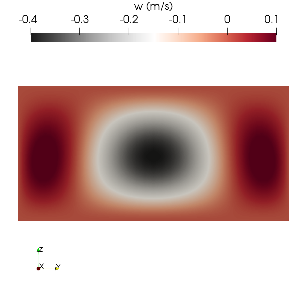
Figure 3. Vertical velocity \(w\) obtained with VERTEX-CFD for \(Ra=5000\) and \(Pr=7\).

6.2 Temperature field

The temperature field evolves from the uniform initial condition of \(200.0\ \mathrm{K}\) toward a statistically steady, convective distribution bounded by the wall temperatures of \(200.0\ \mathrm{K}\) (top) and \(250.0\ \mathrm{K}\) (bottom).

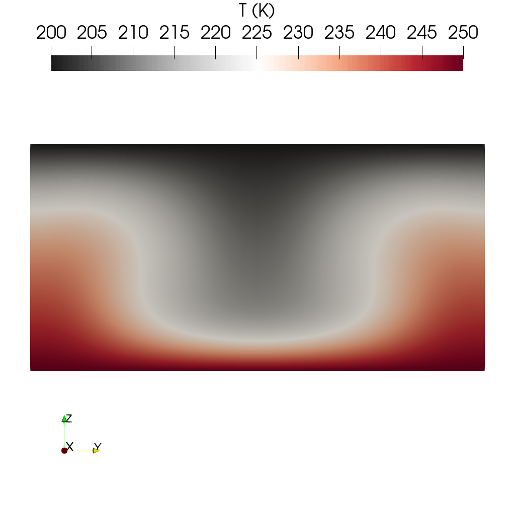
Figure 4. Temperature contours obtained with VERTEX-CFD for \(Ra=5000\) and \(Pr=7\).

[LLC+22]

Pan-Xin Li, Ben-Wen Li, Lu Chen, Xue-Yuan Leng, Xiao-Hong Luo, Yang Yu, and Jing-Kui Zhang. 3d dns of laminar rayleigh-bénard convection in a cylinder for incompressible fluid flow. Chinese Journal of Physics, 79:374–394, 2022.